contour properites

Contour Properties

Here we will learn to extract some frequently used properties of objects like Solidity, Equivalent Diameter, Mask image, Mean Intensity etc. More features can be found at Matlab regionprops documentation.

(NB : Centroid, Area, Perimeter etc also belong to this category, but we have seen it in last chapter)

1. Aspect Ratio  長寬比

It is the ratio of width to height of bounding rect of the object.

x,y,w,h = cv2.boundingRect(cnt)
aspect_ratio = float(w)/h

2. Extent  :  面積比率

Extent is the ratio of contour area to bounding rectangle area.

area = cv2.contourArea(cnt)
x,y,w,h = cv2.boundingRect(cnt)
rect_area = w*h
extent = float(area)/rect_area

3. Solidity

Solidity is the ratio of contour area to its convex hull area.

area = cv2.contourArea(cnt)
hull = cv2.convexHull(cnt)
hull_area = cv2.contourArea(hull)
solidity = float(area)/hull_area

4. Equivalent Diameter

Equivalent Diameter is the diameter of the circle whose area is same as the contour area.

area = cv2.contourArea(cnt)
equi_diameter = np.sqrt(4*area/np.pi)

5. Orientation

Orientation is the angle at which object is directed. Following method also gives the Major Axis and Minor Axis lengths.

(x,y),(MA,ma),angle = cv2.fitEllipse(cnt)

6. Mask and Pixel Points

In some cases, we may need all the points which comprises that object. It can be done as follows:

mask = np.zeros(imgray.shape,np.uint8)
cv2.drawContours(mask,[cnt],0,255,-1)
pixelpoints = np.transpose(np.nonzero(mask))
#pixelpoints = cv2.findNonZero(mask)

Here, two methods, one using Numpy functions, next one using OpenCV function (last commented line) are given to do the same. Results are also same, but with a slight difference. Numpy gives coordinates in (row, column) format, while OpenCV gives coordinates in (x,y) format. So basically the answers will be interchanged. Note that, row = x andcolumn = y.

7. Maximum Value, Minimum Value and their locations

We can find these parameters using a mask image.

min_val, max_val, min_loc, max_loc = cv2.minMaxLoc(imgray,mask = mask)

8. Mean Color or Mean Intensity

Here, we can find the average color of an object. Or it can be average intensity of the object in grayscale mode. We again use the same mask to do it.

mean_val = cv2.mean(im,mask = mask)

9. Extreme Points

Extreme Points means topmost, bottommost, rightmost and leftmost points of the object.

leftmost = tuple(cnt[cnt[:,:,0].argmin()][0])
rightmost = tuple(cnt[cnt[:,:,0].argmax()][0])
topmost = tuple(cnt[cnt[:,:,1].argmin()][0])
bottommost = tuple(cnt[cnt[:,:,1].argmax()][0])

For eg, if I apply it to an Indian map, I get the following result :

Reference : http://docs.opencv.org/3.0-beta/doc/py_tutorials/py_imgproc/py_contours/py_contour_properties/py_contour_properties.html#contour-properties

contour feature

//  sample code

import sys
sys.path.append('/usr/local/lib/python2.7/site-packages')

import numpy as np
import cv2

im = cv2.imread('out077.jpg')
imgray = cv2.cvtColor(im,cv2.COLOR_BGR2GRAY)
ret,thresh = cv2.threshold(imgray,127,255,0)
dst ,contours, hierarchy = cv2.findContours(thresh,cv2.RETR_TREE,cv2.CHAIN_APPROX_SIMPLE)

#cv2.drawContours(im, contours, -1, (0,255,0), 3)
#cv2.drawContours(im, contours, 3, (0,255,0), 3)
#cnt = contours[4]
#cv2.drawContours(im, [cnt], 0, (0,255,0), 3)


for i in range(len(contours)):
        cnt = contours[i]
        M = cv2.moments(cnt)
        #print "total cnt :" + str(cnt)
        area = cv2.contourArea(cnt)

        perimeter = cv2.arcLength(cnt,True)

        x,y,w,h = cv2.boundingRect(cnt)

        cx = int(M['m10']/M['m00'])
        cy = int(M['m01']/M['m00'])


        #if( i== 5):
        if( (area > 400) & ((h > 50) or (w > 50))):
            print "area : " + str(area)
            print "arc length :" + str(perimeter)
            print "w : " + str(w) + " h :" + str(h)
            #cv2.circle(im,(cx,cy),20,(255,0,255),3)
            #cv2.rectangle(im,(x,y),(x+w,y+h),(0,255,0),2)
            ellipse = cv2.fitEllipse(cnt)
            cv2.ellipse(im,ellipse,(0,255,0),2)
            (x,y),radius = cv2.minEnclosingCircle(cnt)
            center = (int(x),int(y))
            radius = int(radius)
            print "radius :" + str(radius)
            cv2.circle(im,center,radius,(0,255,0),2)

            rect = cv2.minAreaRect(cnt)
            box = cv2.boxPoints(rect)
            box = np.int0(box)
            cv2.drawContours(im,[box],0,(0,0,255),2)
            break


cv2.imshow('image',im)
cv2.waitKey(0)
cv2.destroyAllWindows()

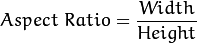
Contour Features

Goal

In this article, we will learn

• To find the different features of contours, like area, perimeter, centroid, bounding box etc
• You will see plenty of functions related to contours.

1. Moments

Image moments help you to calculate some features like center of mass of the object, area of the object etc. Check out the wikipedia page on Image Moments

The function cv2.moments() gives a dictionary of all moment values calculated. See below:

import cv2
import numpy as np

img = cv2.imread('star.jpg',0)
ret,thresh = cv2.threshold(img,127,255,0)
contours,hierarchy = cv2.findContours(thresh, 1, 2)

cnt = contours[0]
M = cv2.moments(cnt)
print M

From this moments, you can extract useful data like area, centroid etc. Centroid is given by the relations, and . This can be done as follows:

cx = int(M['m10']/M['m00'])   中心點 x
cy = int(M['m01']/M['m00'])   中心點 y

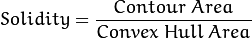
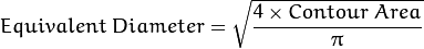
2. Contour Area

Contour area is given by the function cv2.contourArea() or from moments, M[‘m00’].

area = cv2.contourArea(cnt)

3. Contour Perimeter   曲線長度

It is also called arc length. It can be found out using cv2.arcLength() function. Second argument specify whether shape is a closed contour (if passed True), or just a curve.

perimeter = cv2.arcLength(cnt,True)

4. Contour Approximation  曲線內縮

It approximates a contour shape to another shape with less number of vertices depending upon the precision we specify. It is an implementation of Douglas-Peucker algorithm. Check the wikipedia page for algorithm and demonstration.

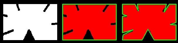
To understand this, suppose you are trying to find a square in an image, but due to some problems in the image, you didn’t get a perfect square, but a “bad shape” (As shown in first image below). Now you can use this function to approximate the shape. In this, second argument is called epsilon, which is maximum distance from contour to approximated contour. It is an accuracy parameter. A wise selection of epsilon is needed to get the correct output.

epsilon = 0.1*cv2.arcLength(cnt,True)
approx = cv2.approxPolyDP(cnt,epsilon,True)

Below, in second image, green line shows the approximated curve for epsilon = 10% of arc length. Third image shows the same for epsilon = 1% of the arc length. Third argument specifies whether curve is closed or not.

5. Convex Hull 曲線外張

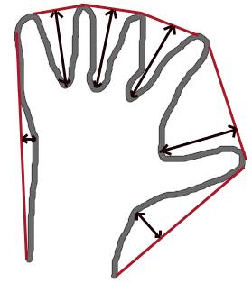
Convex Hull will look similar to contour approximation, but it is not (Both may provide same results in some cases). Here, cv2.convexHull() function checks a curve for convexity defects and corrects it. Generally speaking, convex curves are the curves which are always bulged out, or at-least flat. And if it is bulged inside, it is called convexity defects. For example, check the below image of hand. Red line shows the convex hull of hand. The double-sided arrow marks shows the convexity defects, which are the local maximum deviations of hull from contours.

There is a little bit things to discuss about it its syntax:

hull = cv2.convexHull(points[, hull[, clockwise[, returnPoints]]

Arguments details:

• points are the contours we pass into.
• hull is the output, normally we avoid it.
• clockwise : Orientation flag. If it is True, the output convex hull is oriented clockwise. Otherwise, it is oriented counter-clockwise.
• returnPoints : By default, True. Then it returns the coordinates of the hull points. If False, it returns the indices of contour points corresponding to the hull points.

So to get a convex hull as in above image, following is sufficient:

hull = cv2.convexHull(cnt)

But if you want to find convexity defects, you need to pass returnPoints = False. To understand it, we will take the rectangle image above. First I found its contour as cnt. Now I found its convex hull with returnPoints = True, I got following values: [[[234 202]], [[ 51 202]], [[ 51 79]], [[234 79]]] which are the four corner points of rectangle. Now if do the same with returnPoints = False, I get following result: [[129],[ 67],[ 0],[142]]. These are the indices of corresponding points in contours. For eg, check the first value: cnt[129] = [[234, 202]] which is same as first result (and so on for others).

You will see it again when we discuss about convexity defects.

6. Checking Convexity

There is a function to check if a curve is convex or not, cv2.isContourConvex(). It just return whether True or False. Not a big deal.

k = cv2.isContourConvex(cnt)

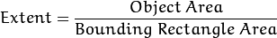
7. Bounding Rectangle

There are two types of bounding rectangles.

7.a. Straight Bounding Rectangle

It is a straight rectangle, it doesn’t consider the rotation of the object. So area of the bounding rectangle won’t be minimum. It is found by the function cv2.boundingRect().

Let (x,y) be the top-left coordinate of the rectangle and (w,h) be its width and height.

x,y,w,h = cv2.boundingRect(cnt)
cv2.rectangle(img,(x,y),(x+w,y+h),(0,255,0),2)

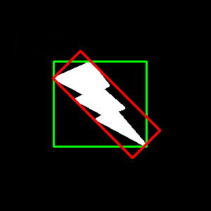
7.b. Rotated Rectangle

Here, bounding rectangle is drawn with minimum area, so it considers the rotation also. The function used iscv2.minAreaRect(). It returns a Box2D structure which contains following detals - ( center (x,y), (width, height), angle of rotation ). But to draw this rectangle, we need 4 corners of the rectangle. It is obtained by the function cv2.boxPoints()

rect = cv2.minAreaRect(cnt)
box = cv2.boxPoints(rect)
box = np.int0(box)
cv2.drawContours(img,[box],0,(0,0,255),2)

Both the rectangles are shown in a single image. Green rectangle shows the normal bounding rect. Red rectangle is the rotated rect.

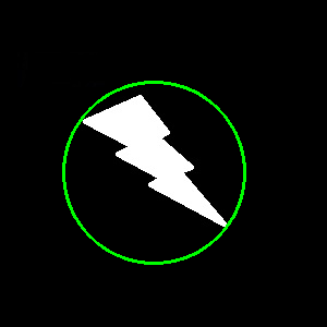
8. Minimum Enclosing Circle

Next we find the circumcircle of an object using the function cv2.minEnclosingCircle(). It is a circle which completely covers the object with minimum area.

(x,y),radius = cv2.minEnclosingCircle(cnt)
center = (int(x),int(y))
radius = int(radius)
cv2.circle(img,center,radius,(0,255,0),2)

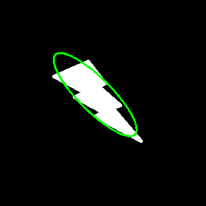
9. Fitting an Ellipse

Next one is to fit an ellipse to an object. It returns the rotated rectangle in which the ellipse is inscribed.

ellipse = cv2.fitEllipse(cnt)
cv2.ellipse(img,ellipse,(0,255,0),2)

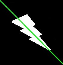
10. Fitting a Line

Similarly we can fit a line to a set of points. Below image contains a set of white points. We can approximate a straight line to it.

rows,cols = img.shape[:2]
[vx,vy,x,y] = cv2.fitLine(cnt, cv2.DIST_L2,0,0.01,0.01)
lefty = int((-x*vy/vx) + y)
righty = int(((cols-x)*vy/vx)+y)
cv2.line(img,(cols-1,righty),(0,lefty),(0,255,0),2)

Reference : http://docs.opencv.org/3.0-beta/doc/py_tutorials/py_imgproc/py_contours/py_contour_features/py_contour_features.html#contour-features

contour getting start

Contours : Getting Started

Goal

• Understand what contours are.
• Learn to find contours, draw contours etc
• You will see these functions : cv2.findContours(), cv2.drawContours()

import numpy as np
import cv2

im = cv2.imread('test.jpg')
imgray = cv2.cvtColor(im,cv2.COLOR_BGR2GRAY)
ret,thresh = cv2.threshold(imgray,127,255,0)
dst , contours, hierarchy = cv2.findContours(thresh,cv2.RETR_TREE,cv2.CHAIN_APPROX_SIMPLE)

To draw all the contours in an image:


cv2.drawContours(img, contours, -1, (0,255,0), 3)

To draw an individual contour, say 4th contour:

cv2.drawContours(img, contours, 3, (0,255,0), 3)

But most of the time, below method will be useful:


cnt = contours[4]
cv2.drawContours(img, [cnt], 0, (0,255,0), 3)

Reference : http://docs.opencv.org/3.0-beta/doc/py_tutorials/py_imgproc/py_contours/py_contours_begin/py_contours_begin.html#contours-getting-started

Performance Optimization Techniques

Performance Optimization Techniques

There are several techniques and coding methods to exploit maximum performance of Python and Numpy. Only relevant ones are noted here and links are given to important sources. The main thing to be noted here is that, first try to implement the algorithm in a simple manner. Once it is working, profile it, find the bottlenecks and optimize them.

1. Avoid using loops in Python as far as possible, especially double/triple loops etc. They are inherently slow.
2. Vectorize the algorithm/code to the maximum possible extent because Numpy and OpenCV are optimized for vector operations.
3. Exploit the cache coherence.
4. Never make copies of array unless it is needed. Try to use views instead. Array copying is a costly operation.

Even after doing all these operations, if your code is still slow, or use of large loops are inevitable, use additional libraries like Cython to make it faster.

Reference : 

Trackbar as the Color Palette

Goal

• Learn to bind trackbar to OpenCV windows
• You will learn these functions : cv2.getTrackbarPos(), cv2.createTrackbar() etc.

Code Demo

Here we will create a simple application which shows the color you specify. You have a window which shows the color and three trackbars to specify each of B,G,R colors. You slide the trackbar and correspondingly window color changes. By default, initial color will be set to Black.

For cv2.getTrackbarPos() function, first argument is the trackbar name, second one is the window name to which it is attached, third argument is the default value, fourth one is the maximum value and fifth one is the callback function which is executed everytime trackbar value changes. The callback function always has a default argument which is the trackbar position. In our case, function does nothing, so we simply pass.

Another important application of trackbar is to use it as a button or switch. OpenCV, by default, doesn’t have button functionality. So you can use trackbar to get such functionality. In our application, we have created one switch in which application works only if switch is ON, otherwise screen is always black.

import cv2
import numpy as np

def nothing(x):
    pass

# Create a black image, a window
img = np.zeros((300,512,3), np.uint8)
cv2.namedWindow('image')

# create trackbars for color change
cv2.createTrackbar('R','image',0,255,nothing)
cv2.createTrackbar('G','image',0,255,nothing)
cv2.createTrackbar('B','image',0,255,nothing)

# create switch for ON/OFF functionality
switch = '0 : OFF \n1 : ON'
cv2.createTrackbar(switch, 'image',0,1,nothing)

while(1):
    cv2.imshow('image',img)
    k = cv2.waitKey(1) & 0xFF
    if k == 27:
        break

    # get current positions of four trackbars
    r = cv2.getTrackbarPos('R','image')
    g = cv2.getTrackbarPos('G','image')
    b = cv2.getTrackbarPos('B','image')
    s = cv2.getTrackbarPos(switch,'image')

    if s == 0:
        img[:] = 0
    else:
        img[:] = [b,g,r]

cv2.destroyAllWindows()

The screenshot of the application looks like below :

Reference : tp://docs.opencv.org/3.0-beta/doc/py_tutorials/py_gui/py_trackbar/py_trackbar.html#trackbar