optical flow for image motion analysis

opencv 提供兩個範例....

sample 1 :

    # calculate optical flow

    p1, st, err = cv2.calcOpticalFlowPyrLK(old_gray, frame_gray, p0, None, **lk_params)

Python: cv2.calcOpticalFlowPyrLK(prevImg, nextImg, prevPts, nextPts[, status[, err[, winSize[, maxLevel[, criteria[, flags[, minEigThreshold]]]]]]]) → nextPts, status, err

Parameters:

prevImg – first 8-bit input image or pyramid constructed by buildOpticalFlowPyramid(). nextImg – second input image or pyramid of the same size and the same type as prevImg. prevPts – vector of 2D points for which the flow needs to be found; point coordinates must be single-precision floating-point numbers. nextPts – output vector of 2D points (with single-precision floating-point coordinates) containing the calculated new positions of input features in the second image; whenOPTFLOW_USE_INITIAL_FLOW flag is passed, the vector must have the same size as in the input. status – output status vector (of unsigned chars); each element of the vector is set to 1 if the flow for the corresponding features has been found, otherwise, it is set to 0. err – output vector of errors; each element of the vector is set to an error for the corresponding feature, type of the error measure can be set in flags parameter; if the flow wasn’t found then the error is not defined (use the status parameter to find such cases). winSize – size of the search window at each pyramid level. maxLevel – 0-based maximal pyramid level number; if set to 0, pyramids are not used (single level), if set to 1, two levels are used, and so on; if pyramids are passed to input then algorithm will use as many levels as pyramids have but no more than maxLevel. criteria – parameter, specifying the termination criteria of the iterative search algorithm (after the specified maximum number of iterations criteria.maxCount or when the search window moves by less than criteria.epsilon. flags – operation flags: OPTFLOW_USE_INITIAL_FLOW uses initial estimations, stored in nextPts; if the flag is not set, then prevPts is copied to nextPts and is considered the initial estimate. OPTFLOW_LK_GET_MIN_EIGENVALS use minimum eigen values as an error measure (seeminEigThreshold description); if the flag is not set, then L1 distance between patches around the original and a moved point, divided by number of pixels in a window, is used as a error measure. minEigThreshold – the algorithm calculates the minimum eigen value of a 2x2 normal matrix of optical flow equations (this matrix is called a spatial gradient matrix in [Bouguet00]), divided by number of pixels in a window; if this value is less than minEigThreshold, then a corresponding feature is filtered out and its flow is not processed, so it allows to remove bad points and get a performance boost.

Sample 2:

cv2.calcOpticalFlowFarneback(prvs,next, None, 0.5, 3, 15, 3, 5, 1.2, 0)

Python: cv2.calcOpticalFlowFarneback(prev, next, flow, pyr_scale, levels, winsize, iterations, poly_n, poly_sigma, flags)→ flow

Parameters:

prev – first 8-bit single-channel input image. next – second input image of the same size and the same type as prev. flow – computed flow image that has the same size as prev and type CV_32FC2. pyr_scale – parameter, specifying the image scale (<1) to build pyramids for each image;pyr_scale=0.5 means a classical pyramid, where each next layer is twice smaller than the previous one. levels – number of pyramid layers including the initial image; levels=1 means that no extra layers are created and only the original images are used. winsize – averaging window size; larger values increase the algorithm robustness to image noise and give more chances for fast motion detection, but yield more blurred motion field. iterations – number of iterations the algorithm does at each pyramid level. poly_n – size of the pixel neighborhood used to find polynomial expansion in each pixel; larger values mean that the image will be approximated with smoother surfaces, yielding more robust algorithm and more blurred motion field, typically poly_n =5 or 7. poly_sigma – standard deviation of the Gaussian that is used to smooth derivatives used as a basis for the polynomial expansion; for poly_n=5, you can set poly_sigma=1.1, for poly_n=7, a good value would be poly_sigma=1.5. flags –

Optical Flow

Goal

In this chapter,

• We will understand the concepts of optical flow and its estimation using Lucas-Kanade method.
• We will use functions like cv2.calcOpticalFlowPyrLK() to track feature points in a video.

Optical Flow

Optical flow is the pattern of apparent motion of image objects between two consecutive frames caused by the movemement of object or camera. It is 2D vector field where each vector is a displacement vector showing the movement of points from first frame to second. Consider the image below (Image Courtesy: Wikipedia article on Optical Flow).

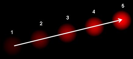
It shows a ball moving in 5 consecutive frames. The arrow shows its displacement vector. Optical flow has many applications in areas like :

• Structure from Motion
• Video Compression
• Video Stabilization ...

Optical flow works on several assumptions:

1. The pixel intensities of an object do not change between consecutive frames.
2. Neighbouring pixels have similar motion.

Consider a pixel  in first frame (Check a new dimension, time, is added here. Earlier we were working with images only, so no need of time). It moves by distance  in next frame taken after  time. So since those pixels are the same and intensity does not change, we can say,

Then take taylor series approximation of right-hand side, remove common terms and divide by  to get the following equation: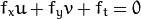

where:

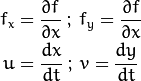
Above equation is called Optical Flow equation. In it, we can find  and , they are image gradients. Similarly  is the gradient along time. But  is unknown. We cannot solve this one equation with two unknown variables. So several methods are provided to solve this problem and one of them is Lucas-Kanade.

Lucas-Kanade method

We have seen an assumption before, that all the neighbouring pixels will have similar motion. Lucas-Kanade method takes a 3x3 patch around the point. So all the 9 points have the same motion. We can find  for these 9 points. So now our problem becomes solving 9 equations with two unknown variables which is over-determined. A better solution is obtained with least square fit method. Below is the final solution which is two equation-two unknown problem and solve to get the solution.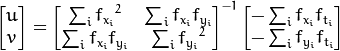

( Check similarity of inverse matrix with Harris corner detector. It denotes that corners are better points to be tracked.)

So from user point of view, idea is simple, we give some points to track, we receive the optical flow vectors of those points. But again there are some problems. Until now, we were dealing with small motions. So it fails when there is large motion. So again we go for pyramids. When we go up in the pyramid, small motions are removed and large motions becomes small motions. So applying Lucas-Kanade there, we get optical flow along with the scale.

Lucas-Kanade Optical Flow in OpenCV

OpenCV provides all these in a single function, cv2.calcOpticalFlowPyrLK(). Here, we create a simple application which tracks some points in a video. To decide the points, we use cv2.goodFeaturesToTrack(). We take the first frame, detect some Shi-Tomasi corner points in it, then we iteratively track those points using Lucas-Kanade optical flow. For the function cv2.calcOpticalFlowPyrLK() we pass the previous frame, previous points and next frame. It returns next points along with some status numbers which has a value of 1 if next point is found, else zero. We iteratively pass these next points as previous points in next step. See the code below:

import numpy as np
import cv2

cap = cv2.VideoCapture('slow.flv')

# params for ShiTomasi corner detection
feature_params = dict( maxCorners = 100,
                       qualityLevel = 0.3,
                       minDistance = 7,
                       blockSize = 7 )

# Parameters for lucas kanade optical flow
lk_params = dict( winSize  = (15,15),
                  maxLevel = 2,
                  criteria = (cv2.TERM_CRITERIA_EPS | cv2.TERM_CRITERIA_COUNT, 10, 0.03))

# Create some random colors
color = np.random.randint(0,255,(100,3))

# Take first frame and find corners in it
ret, old_frame = cap.read()
old_gray = cv2.cvtColor(old_frame, cv2.COLOR_BGR2GRAY)
p0 = cv2.goodFeaturesToTrack(old_gray, mask = None, **feature_params)

# Create a mask image for drawing purposes
mask = np.zeros_like(old_frame)

while(1):
    ret,frame = cap.read()
    frame_gray = cv2.cvtColor(frame, cv2.COLOR_BGR2GRAY)

    # calculate optical flow
    p1, st, err = cv2.calcOpticalFlowPyrLK(old_gray, frame_gray, p0, None, **lk_params)

    # Select good points
    good_new = p1[st==1]
    good_old = p0[st==1]

    # draw the tracks
    for i,(new,old) in enumerate(zip(good_new,good_old)):
        a,b = new.ravel()
        c,d = old.ravel()
        mask = cv2.line(mask, (a,b),(c,d), color[i].tolist(), 2)
        frame = cv2.circle(frame,(a,b),5,color[i].tolist(),-1)
    img = cv2.add(frame,mask)

    cv2.imshow('frame',img)
    k = cv2.waitKey(30) & 0xff
    if k == 27:
        break

    # Now update the previous frame and previous points
    old_gray = frame_gray.copy()
    p0 = good_new.reshape(-1,1,2)

cv2.destroyAllWindows()
cap.release()

Dense Optical Flow in OpenCV

Lucas-Kanade method computes optical flow for a sparse feature set (in our example, corners detected using Shi-Tomasi algorithm). OpenCV provides another algorithm to find the dense optical flow. It computes the optical flow for all the points in the frame. It is based on Gunner Farneback’s algorithm which is explained in “Two-Frame Motion Estimation Based on Polynomial Expansion” by Gunner Farneback in 2003.

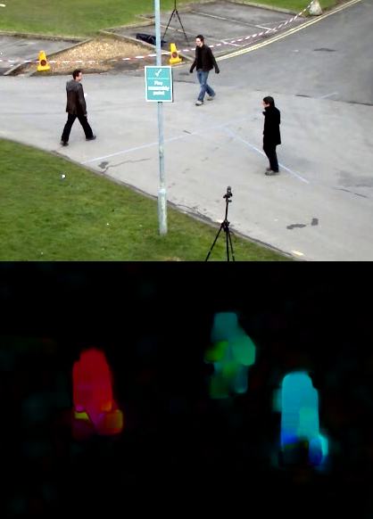
Below sample shows how to find the dense optical flow using above algorithm. We get a 2-channel array with optical flow vectors, . We find their magnitude and direction. We color code the result for better visualization. Direction corresponds to Hue value of the image. Magnitude corresponds to Value plane. See the code below:

import cv2
import numpy as np
cap = cv2.VideoCapture("vtest.avi")

ret, frame1 = cap.read()
prvs = cv2.cvtColor(frame1,cv2.COLOR_BGR2GRAY)
hsv = np.zeros_like(frame1)
hsv[...,1] = 255

while(1):
    ret, frame2 = cap.read()
    next = cv2.cvtColor(frame2,cv2.COLOR_BGR2GRAY)

    flow = cv2.calcOpticalFlowFarneback(prvs,next, None, 0.5, 3, 15, 3, 5, 1.2, 0)

    mag, ang = cv2.cartToPolar(flow[...,0], flow[...,1])
    hsv[...,0] = ang*180/np.pi/2
    hsv[...,2] = cv2.normalize(mag,None,0,255,cv2.NORM_MINMAX)
    rgb = cv2.cvtColor(hsv,cv2.COLOR_HSV2BGR)

    cv2.imshow('frame2',rgb)
    k = cv2.waitKey(30) & 0xff
    if k == 27:
        break
    elif k == ord('s'):
        cv2.imwrite('opticalfb.png',frame2)
        cv2.imwrite('opticalhsv.png',rgb)
    prvs = next

cap.release()
cv2.destroyAllWindows()

See the result below:

OpenCV comes with a more advanced sample on dense optical flow, please see samples/python2/opt_flow.py.

Reference : http://docs.opencv.org/3.0-beta/doc/py_tutorials/py_video/py_lucas_kanade/py_lucas_kanade.html#lucas-kanade

Reference : http://docs.opencv.org/3.0-beta/modules/video/doc/motion_analysis_and_object_tracking.html